Game Sales Analysis Final Project: Finding the Ideal Genre

Introduction

This project utilizes video game sales data from Kaggle to solve a potential business decision made by a fictional game studio. View the slide deck covering the same topics and a video walkthrough from the link in the sidebar.

Background

A fictional video game studio has been getting by for a few years producing low-budget fighting games. Recently, they had the opportunity for a new investor to get involved in their product and have a much higher budget for their next title. However, they also have a much higher sales target than in the past.

Problem

This studio has generally tended towards making fighting games. However, they now need to hit a sales target of 1.5 million copies to continue running, so they have decided to investigate if making a game of a different genre would help them reach this goal. Although this is the highest priority, there is a second goal of getting their game into the top 5 best-sellers of its genre in its release year. This would give them a solid chance at awards and critical acclaim that may help them get funding for future titles.

Exploratory Analysis

Before conducting the analysis of our specific problem, we must better understand the data we are working with. The game sales dataset has eleven different variables, and each entry represents a single release of a game that sold at least ten thousand copies worldwide. The attributes of these entries include the game’s name, its genre, the publisher that released it, the platform it was released on, five different sales columns representing the total copies sold in North America, Europe, Japan, other regions, and the whole world, the year of the game’s release, and the overal global sales ranking of a game in the dataset.

This dataset does not comprehensively cover all of the video game sales data that would be desired to make an informed decision regarding genre of a new game being produced today, as games released over the last eight years are not included and recent video game consoles are missing from the platforms as well. However, an updated version of this dataset could be analyzed in the same way as the limited dataset in this article, so the existing data is being used as a proof-of-concept of exploratory and business analysis.

Categorical Data

Genre

Code

missing_genre <- game_sales |>
  filter(is.na(genre)) |>
  summarize(count = n()) |>
  pluck("count")

paste("Number of entries missing genre:",missing_genre)

[1] "Number of entries missing genre: 0"

Code

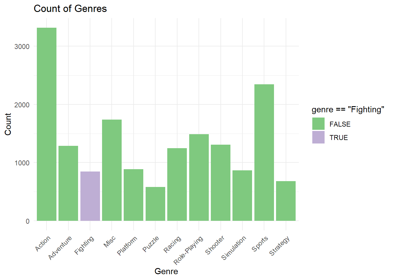
genre_groups <- game_sales |>
  group_by(genre) |>
  summarize(count = n())

genre_groups |>
  ggplot() +
  geom_col(mapping = aes(x = genre, y = count, fill = genre == "Fighting")) +
  scale_fill_brewer(palette = "Accent") +
  theme_minimal() +
  theme(axis.text.x = element_text(angle = 45, hjust = 1)) +
  labs(x = "Genre", y = "Count", title = "Count of Genres")

There are twelve genres included in our dataset, one of them being Fighting–the genre the development studio was most interested in producing. By far the most common games in this dataset are Action games, followed by Sports games, and the least popular are Puzzle and Strategy, although there may be some overlap between these categories. There is a Misc category as a catch-all, so there are no games missing a genre in the dataset.

Publisher

Code

missing_publisher <- game_sales |>
  filter(is.na(publisher)) |>
  summarize(count = n()) |>
  pluck("count")

total_publishers <- game_sales |>
  pluck("publisher") |>
  unique() |>
  length()

paste("Number of entries missing publisher:",missing_publisher)

[1] "Number of entries missing publisher: 58"

Code

paste("Number of unique publishers in the dataset:",total_publishers)

[1] "Number of unique publishers in the dataset: 579"

Code

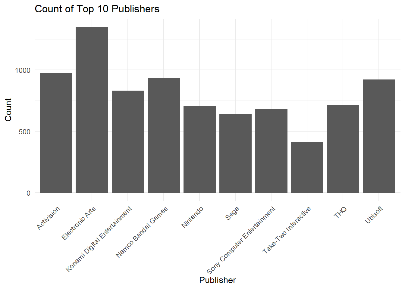
top_publishers <- game_sales |>
  group_by(publisher) |>
  summarize(count = n()) |>
  slice_max(count, n = 10)

top_publishers |>
  ggplot() +
  geom_col(mapping = aes(x = publisher, y = count)) + 
  theme_minimal() +
  theme(axis.text.x = element_text(angle = 45, hjust = 1)) +
  labs(x = "Publisher", y = "Count", title = "Count of Top 10 Publishers")

Unlike genre, there are some entries in the dataset that are missing information about who published them. Whether these are cases where actual ownership over the game is unclear due to changing publishers or the source the data was pulled from was simply missing the publisher by mistake is unclear. With over 500 publishers, we cannot visualize how common each one is, so we will instead view the top 10. The most common publisher in the entire dataset is Electronic Arts, followed by Activision, Namco Bandai Games, and Ubisoft.

Code

total_game_count <- game_sales |>
  summarize(count = n()) |>
  pluck("count")

top_publisher_game_count <- game_sales |>
  filter(publisher %in% top_publishers$publisher) |>
  summarize(count = n()) |>
  pluck("count")

paste("Total number of games published by top 10 publishers:",top_publisher_game_count)

[1] "Total number of games published by top 10 publishers: 8164"

Code

paste("Percentage of games in dataset published by top 10 publishers:",round(100*top_publisher_game_count/total_game_count, 2),"%")

[1] "Percentage of games in dataset published by top 10 publishers: 49.19 %"

These top 10 publishers have published nearly 50% of the total games in the dataset, even though there are over 500 other publishers included. Further analysis could give an idea of how successful these games by big-name publishers tend to be compared to other publishers that might be ‘one-hit wonders’.

Platform

Code

missing_platform <- game_sales |>
  filter(is.na(platform)) |>
  summarize(count = n()) |>
  pluck("count")

total_platforms <- game_sales |>
  pluck("platform") |>
  unique() |>
  length()

paste("Number of entries missing platform:",missing_platform)

[1] "Number of entries missing platform: 0"

Code

paste("Number of unique platforms in the dataset:",total_platforms)

[1] "Number of unique platforms in the dataset: 31"

Code

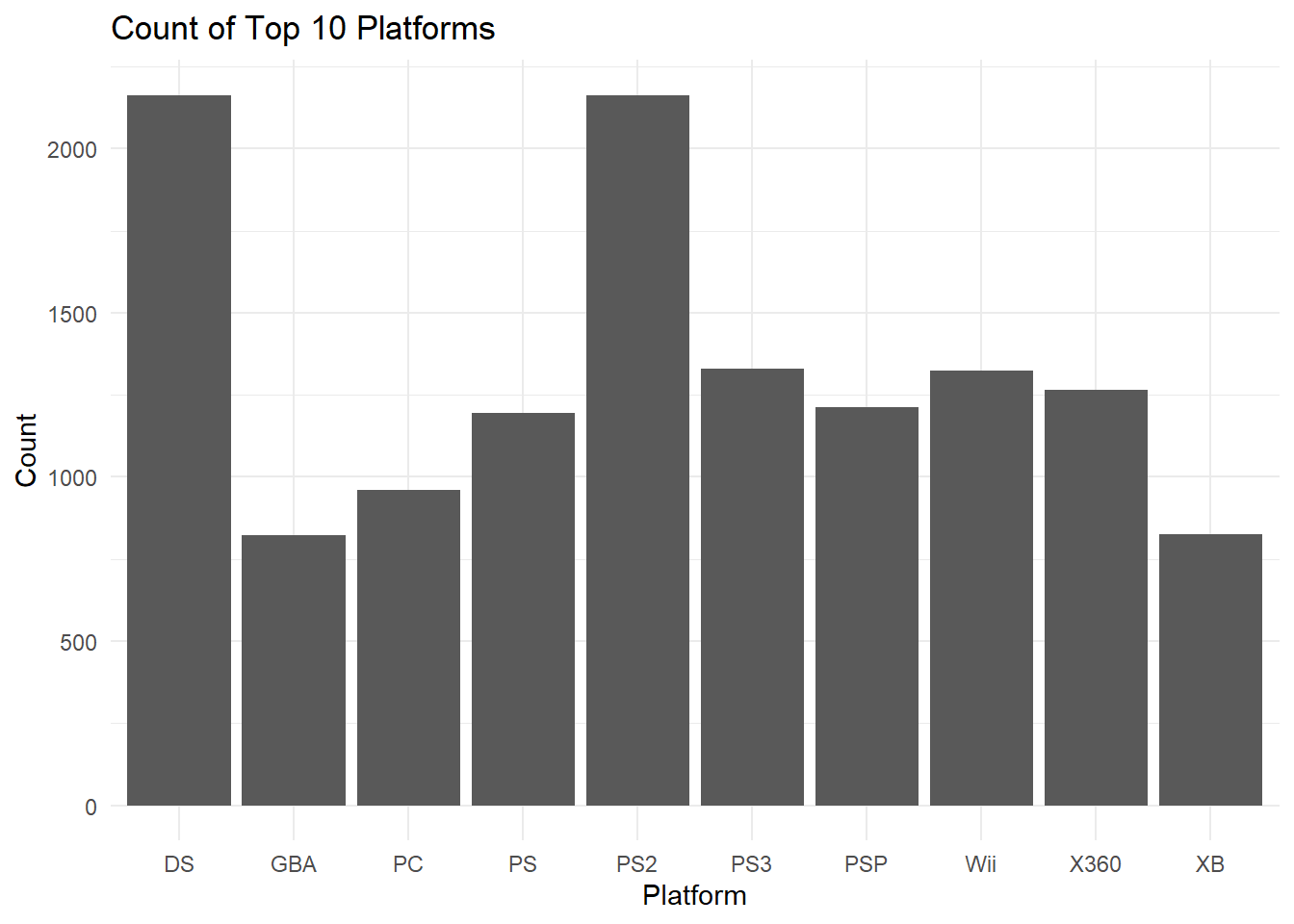
top_platforms <- game_sales |>
  group_by(platform) |>
  summarize(count = n()) |>
  slice_max(count, n = 10)

top_platforms |>
  ggplot() +
  geom_col(mapping = aes(x = platform, y = count)) +
  theme_minimal() + 
  labs(x = "Platform", y = "Count", title = "Count of Top 10 Platforms")

Every entry in the dataset has a platform associated with it, of which there are 31 total in the dataset. The top two platforms, the DS and the PS2 are extremely close in number of games, and they both have over a 500 game lead compared to the next most popular platforms.

Code

top_platform_game_count <- game_sales |>
  filter(platform %in% top_platforms$platform) |>
  summarize(count = n()) |>
  pluck("count")

paste("Total number of games released on top 10 platforms:",top_platform_game_count)

[1] "Total number of games released on top 10 platforms: 13258"

Code

paste("Percentage of games in dataset released on top 10 platforms:",round(100*top_platform_game_count/total_game_count, 2),"%")

[1] "Percentage of games in dataset released on top 10 platforms: 79.88 %"

These top 10 platforms make up a very large portion of the games in the dataset–nearly 80%. However, unlike game publishing companies that persist over time, many platforms grow out-of-date as new consoles are released. Rather than focus too much on the individual platform, later analysis could categorize platforms by the company that produced them and anaylyze the success of games released on them.

Continuous Data

Years

Code

missing_year <- game_sales |>
  filter(is.na(year)) |>
  summarize(count = n()) |>
  pluck("count")

paste("Number of entries missing year:",missing_year)

[1] "Number of entries missing year: 271"

Code

game_sales |>
  arrange(year) |>
  pluck("year") |>
  unique()

 [1] 1980 1981 1982 1983 1984 1985 1986 1987 1988 1989 1990 1991 1992 1993 1994
[16] 1995 1996 1997 1998 1999 2000 2001 2002 2003 2004 2005 2006 2007 2008 2009
[31] 2010 2011 2012 2013 2014 2015 2016 2017 2020   NA

Code

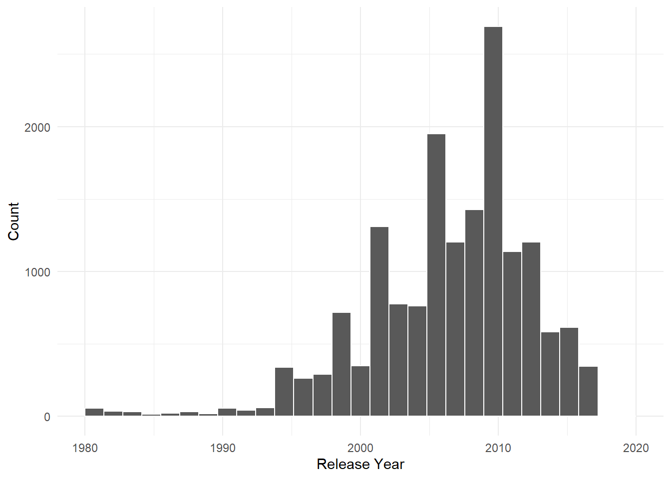
game_sales |>
  ggplot() +
  geom_histogram(mapping = aes(x = year), color = 'white') +
  theme_minimal() +
  labs(x = "Release Year", y = "Count")

There are quite a few games missing release year in the dataset, which starts as early as 1980. It continues up to 2017 with a peak around 2010, then strangely skips two years and has a very small amount of data again in 2020. Time series modeling will not be relevant for this analysis, but these discrepancies with the data are good to keep in mind.

Sales

Code

global_range <- game_sales |>
  pluck("global_sales") |>
  range()

na_range <- game_sales |>
  pluck("na_sales") |>
  range()

eu_range <- game_sales |>
  pluck("eu_sales") |>
  range()

jp_range <- game_sales |>
  pluck("jp_sales") |>
  range()

other_range <- game_sales |>
  pluck("other_sales") |>
  range()

paste("Range of Global sales:",global_range[1],"-",global_range[2])

[1] "Range of Global sales: 0.01 - 82.74"

Code

paste("Range of North America sales:",na_range[1],"-",na_range[2])

[1] "Range of North America sales: 0 - 41.49"

Code

paste("Range of Europe sales:",eu_range[1],"-",eu_range[2])

[1] "Range of Europe sales: 0 - 29.02"

Code

paste("Range of Japan sales:",jp_range[1],"-",jp_range[2])

[1] "Range of Japan sales: 0 - 10.22"

Code

paste("Range of Other sales:",other_range[1],"-",other_range[2])

[1] "Range of Other sales: 0 - 10.57"

There are five different sales columns in the dataset: three specific regions, one catch-all column for copies sold in other regions, and a global sales column that sums the total copies sold across all regions, all of which are in millions. The minimum required sales to be in this dataset is 10 thousand, so the minimum global sales value is .01, but it is common for a game that is successful in one region to remain unpopular or not be released in another, so all of the more specific sales columns go all the way down to 0. Naturally the highest-reaching column is the sum global sales, but of the separate regions, North America has the highest sales, followed by Europe, the ‘Other’ region, and Japan.

Code

game_sales |>
  ggplot() +
  geom_point(mapping = aes(x = year, y = global_sales)) +
  theme_minimal() + 
  labs(x = 'Release Year', y = 'Global Copies Sold (Millions)')

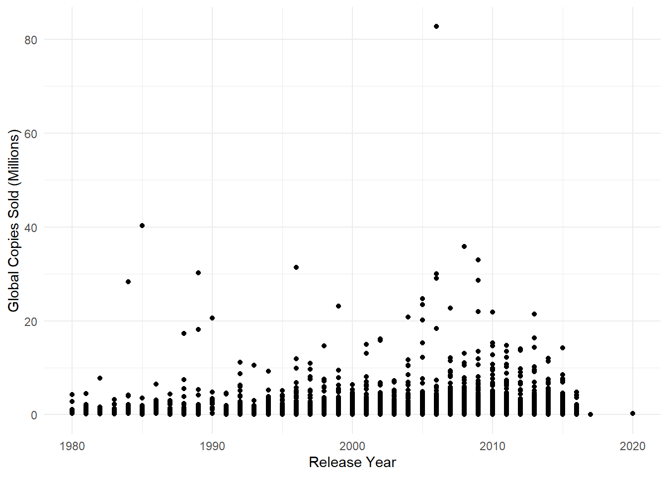
Looking at the number of copies sold globally throughout the dataset, we can see that the data is extremely heavily 0-weighted, or 0.1-weighted when it comes to the global sales column, as expected with count data. However, there are a handful of extremely high-selling games that are included in the dataset as well.

Business Analysis

Meeting Sales Target

Designing Metric

Now that we understand what variables are available in our dataset, we can utilize them to create a useful metric for the primary business goal. This is done by adding a new column of boolean values, noting if a game met the target set by the studio or not.

Code

game_sales <- game_sales |>
  mutate(meets_target = ifelse(global_sales >= 1.5, 1, 0))

Code

genre_target_ratios <- game_sales |>
  group_by(genre) |>
  summarize(meets_target_ratio = mean(meets_target)) |>
  arrange(desc(meets_target_ratio))

Graphing Genres and Meeting Target Sales Percentage

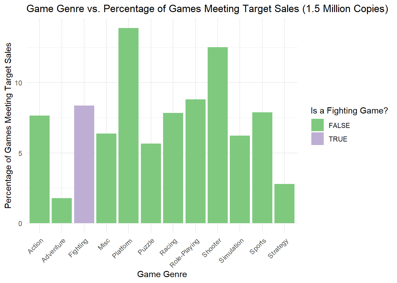
By graphing the percentage of games meeting the target of 1.5 million copies sold, we see that a fighting game may not be the best choice. Role-playing games seem to be a slight improvement, and platformer and shooter games appear to be about 5% more likely to meet such a sales target. It is very possible that there is a confounding variable linking the genre and global sales values, such as the average price of different genres of games, but this is not present in our data. Thus, we will only investigate the significance of the connection between genre and meeting target sales directly.

Code

genre_target_ratios |>
  mutate(meets_target_percent = meets_target_ratio * 100) |>
  ggplot() +
  geom_col(mapping = aes(x = genre, y = meets_target_percent, fill = genre == "Fighting")) +
  theme_minimal() +
  labs (x = "Game Genre", y = "Percentage of Games Meeting Target Sales", title = "Game Genre vs. Percentage of Games Meeting Target Sales (1.5 Million Copies)", fill = "Is a Fighting Game?") +
  scale_fill_brewer(palette = "Accent") +
  theme(axis.text.x = element_text(angle = 45, hjust = 1))

ANOVA Testing

First, we will conduct an ANOVA test to see if it is possible the true population percentage of games meeting target sales is the same across all genres. We get a high F value and a very small P-value, meaning that this data would be extremely unlikely to be collected if this null hypothesis was true. Therefore, we can assume that genre has an impact on the likelihood of a game meeting target sales.

Code

aov_result <- aov(meets_target ~ genre, data = game_sales)
summary(aov_result)

               Df Sum Sq Mean Sq F value Pr(>F)    
genre          11   13.5  1.2287   17.63 <2e-16 ***
Residuals   16586 1155.9  0.0697                   
---
Signif. codes:  0 '***' 0.001 '**' 0.01 '*' 0.05 '.' 0.1 ' ' 1

Fisher’s Exact Hypothesis Testing

Knowing that it is highly unlikely all genres have an equal chance of meeting target sales is useful, but we need to investigate the specific genres that appear to be more successful than the preferred genre, fighting games. We can create three contingency tables, showing the number of ‘successes’ (games that met target sales) and ‘failures’ (games that did not meet target sales) of fighting games and one of three other genres: platformers, shooters, and role-playing games. With the data in this format, we can conduct Fisher’s Exact Test on each table to get an idea of how unlikely it is that games of the two genres under investigation have an equal probability of meeting target sales. If we get a low p-value on a test (for example, less than .05), that is an indicator that there is a difference in the probability of hitting the sales target for the two categories.

Code

fighting_platform_table <- game_sales |>
  filter(genre %in% c("Fighting", "Platform")) |>
  group_by(genre) |>
  summarize(met_target = sum(meets_target), missed_target = n() - met_target)
fighting_platform_table

# A tibble: 2 × 3
  genre    met_target missed_target
  <chr>         <dbl>         <dbl>
1 Fighting         71           777
2 Platform        123           763

Code

fighting_shooter_table <- game_sales |>
  filter(genre %in% c("Fighting", "Shooter")) |>
  group_by(genre) |>
  summarize(met_target = sum(meets_target), missed_target = n() - met_target)
fighting_shooter_table

# A tibble: 2 × 3
  genre    met_target missed_target
  <chr>         <dbl>         <dbl>
1 Fighting         71           777
2 Shooter         164          1146

Code

fighting_roleplaying_table <- game_sales |>
  filter(genre %in% c("Fighting","Role-Playing")) |>
  group_by(genre) |>
  summarize(met_target = sum(meets_target), missed_target = n() - met_target)
fighting_roleplaying_table

# A tibble: 2 × 3
  genre        met_target missed_target
  <chr>             <dbl>         <dbl>
1 Fighting             71           777
2 Role-Playing        131          1357

Code

fisher.test(select(fighting_platform_table, met_target, missed_target))


    Fisher's Exact Test for Count Data

data:  select(fighting_platform_table, met_target, missed_target)
p-value = 0.0003234
alternative hypothesis: true odds ratio is not equal to 1
95 percent confidence interval:
 0.4100787 0.7794299
sample estimates:
odds ratio 
 0.5670237

Code

fisher.test(select(fighting_shooter_table, met_target, missed_target))


    Fisher's Exact Test for Count Data

data:  select(fighting_shooter_table, met_target, missed_target)
p-value = 0.002345
alternative hypothesis: true odds ratio is not equal to 1
95 percent confidence interval:
 0.4693230 0.8622751
sample estimates:
odds ratio 
 0.6386536

Code

fisher.test(select(fighting_roleplaying_table, met_target, missed_target))


    Fisher's Exact Test for Count Data

data:  select(fighting_roleplaying_table, met_target, missed_target)
p-value = 0.7597
alternative hypothesis: true odds ratio is not equal to 1
95 percent confidence interval:
 0.6893464 1.2914795
sample estimates:
odds ratio 
 0.9465713

These results show that it would be very unlikely to find data more extreme than our sample if Fighting and Platform games had the same average global sales value, and the same is true for Fighting and Shooter games. Thus, we can assume that the probability of meeting our sales target is different for these categories. On the other hand, the Fighting and Role-Playing hypothesis test provided a large p-value, so we cannot make the same assumption about these two games. We would expect Role-Playing games to be as likely to be successful as Fighting games.

Now that we have assumed Platform games are more likely to meet the sales target that Fighting games, and likewise with Shooter games and Fighter games, it would be good to know if one of Platform or Shooter games was noticeably better than the other, as this would drive our decision forward. We can follow the same process of creating a contingency table and using Fisher’s Exact Test with Platform and Shooter games.

Code

platform_shooter_table <- game_sales |>
  filter(genre %in% c("Platform","Shooter")) |>
  group_by(genre) |>
  summarize(met_target = sum(meets_target), missed_target = n() - met_target)
platform_shooter_table

# A tibble: 2 × 3
  genre    met_target missed_target
  <chr>         <dbl>         <dbl>
1 Platform        123           763
2 Shooter         164          1146

Code

fisher.test(select(platform_shooter_table, met_target, missed_target))


    Fisher's Exact Test for Count Data

data:  select(platform_shooter_table, met_target, missed_target)
p-value = 0.3666
alternative hypothesis: true odds ratio is not equal to 1
95 percent confidence interval:
 0.8683859 1.4583802
sample estimates:
odds ratio 
   1.12641

The result from this test is insignificant, and thus we cannot conclude that one of Platform and Shooter games has a higher probability of meeting the sales target than the other. Since these two genres both are better at meeting our first goal than Fighting games, we can now investigate our second priority and see if one of the two best options is better there.

Finding Fifth-Best Benchmark

Designing Secondary Metric

The second priority of the team is getting their game into the top 5 best-selling games of its genre for its release year. To make the chances of this more likely, they want to pick a genre with a lower bar to reach to get into the top 5 games of its kind of the year. We can measure this by finding the average number of copies sold of yearly fifth-best-sellers. Since we are only focusing on Platform and Shooter games, we want to find which genre has a lower value on this metric, as that indicates it may be easier for the team to get the game into the top 5.

To calculate our metric, we want to filter our games to one genre (either platformers or shooters), group it by the year, find the fifth best game by global sales of each year, then get the mean of these values. However, in some years there might not have been 5 games sold in our data, so in these cases we will take the lowest ranking game.

Code

fifth_best_platforms <- game_sales |>
  filter(genre == "Platform", !is.na(year)) |>
  group_by(year) |>
  mutate(year_rank = order(order(global_sales, decreasing = TRUE))) |>
  filter(year_rank == ifelse(n() < 5, n(), 5))

fifth_best_shooters <- game_sales |>
  filter(genre == "Shooter", !is.na(year)) |>
  group_by(year) |>
  mutate(year_rank = order(order(global_sales, decreasing = TRUE))) |>
  filter(year_rank == ifelse(n() < 5, n(), 5))

fifth_best_platforms_mean <- fifth_best_platforms |>
  pluck("global_sales") |>
  mean()

paste("Global sales mean of fifth-best platformers: ", round(fifth_best_platforms_mean, 3))

[1] "Global sales mean of fifth-best platformers:  1.222"

Code

fifth_best_shooters_mean <- fifth_best_shooters |>
  pluck("global_sales") |>
  mean()

paste("Global sales mean of fifth-best shooters: ", round(fifth_best_shooters_mean, 3))

[1] "Global sales mean of fifth-best shooters:  1.621"

It appears that the average global sales made by a fifth-best-selling game is higher for a shooter than a platformer, which would imply that a platformer would be easier to get into the top 5 for and thus a better choice. However, the resulting metric for our data is not necessarily the true population value. To get an idea of a range the true metrics may fall into, we can bootstrap our data and use it to help create confidence intervals.

Secondary Metric Bootstrapping

Bootstrapping is a method of simulating random sampling from the population by treating our existing sample as the population and taking samples from it with replacement. To do this, we must assume that our game sales data is representative of the true population of video games. This is not the most accurate assumption, since the data is intended to be comprehensive above a certain point, rather than a random sample of video games. However, this method can still potentially help us estimate what the distribution of random samples of video games could look like.

Code

n_iter <- 10^3

platform_values <- c(NULL)

platform_sales <- game_sales |>
  filter(genre == "Platform")

for (i in 1:n_iter) {
  metric <- slice_sample(platform_sales, n = nrow(platform_sales), replace = TRUE) |>
    group_by(year) |>
    mutate(year_rank = order(order(global_sales, decreasing = TRUE))) |>
    filter(year_rank == ifelse(n() < 5, n(), 5)) |>
    pluck("global_sales") |>
    mean()
  
  platform_values = c(platform_values, metric)
}

Code

shooter_values <- c(NULL)

shooter_sales <- game_sales |>
  filter(genre == "Shooter")

for (i in 1:n_iter) {
  metric <- slice_sample(shooter_sales, n = nrow(shooter_sales), replace = TRUE) |>
    group_by(year) |>
    mutate(year_rank = order(order(global_sales, decreasing = TRUE))) |>
    filter(year_rank == ifelse(n() < 5, n(), 5)) |>
    pluck("global_sales") |>
    mean()
  
  shooter_values = c(shooter_values, metric)
}

Code

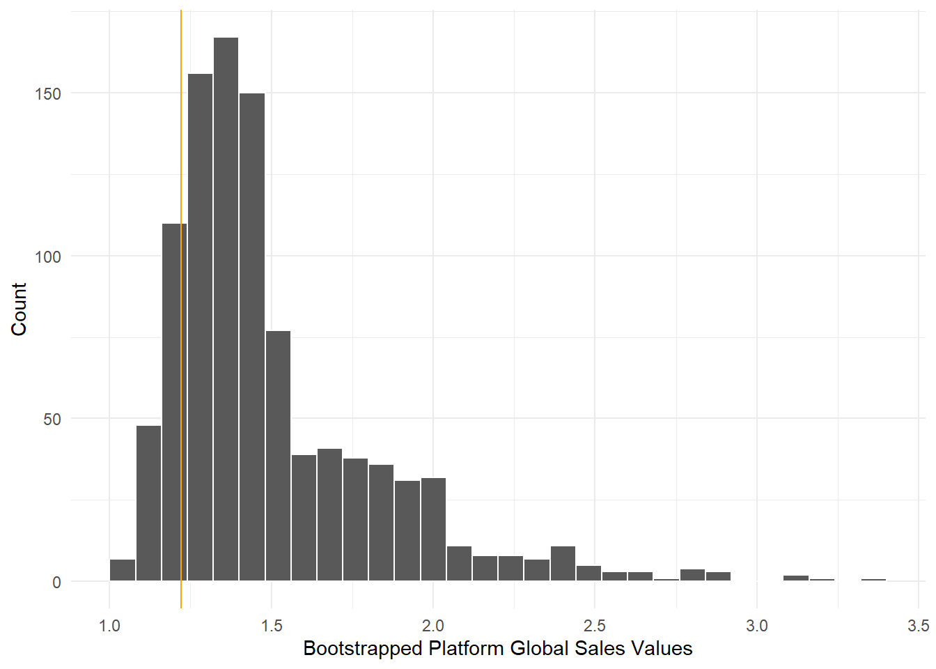
ggplot() +
  geom_histogram(mapping = aes(x = platform_values), color = 'white') +
  geom_vline(xintercept = fifth_best_platforms_mean, color = 'orange') +
  theme_minimal() +
  labs(x = "Bootstrapped Platform Global Sales Values", y = "Count")

Code

platform_se <- sd(platform_values)

Code

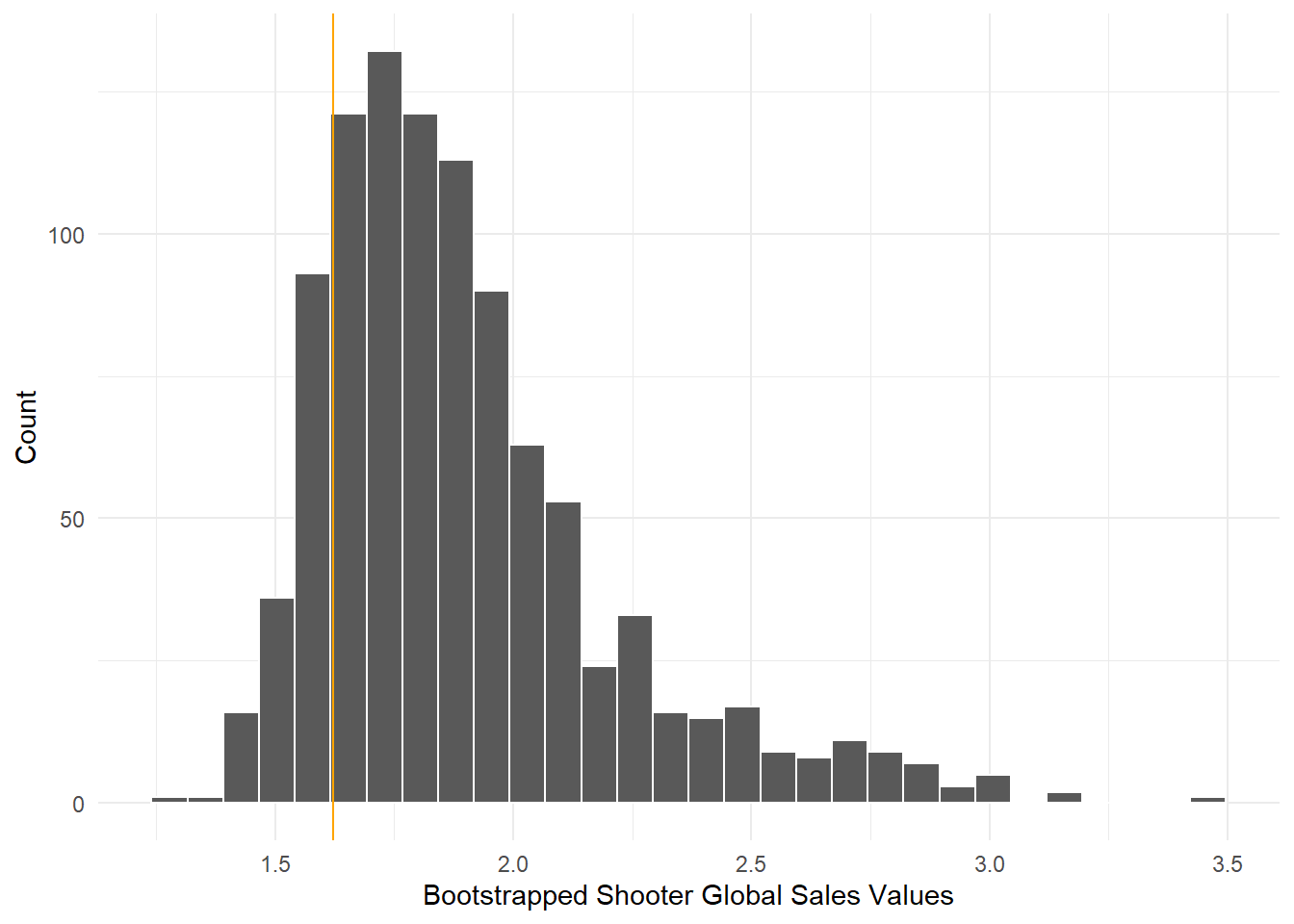
ggplot() +
  geom_histogram(mapping = aes(x = shooter_values), color = 'white') +
  geom_vline(xintercept = fifth_best_shooters_mean, color = 'orange') +
  theme_minimal() +
  labs(x = "Bootstrapped Shooter Global Sales Values", y = "Count")

Code

shooter_se <- sd(shooter_values)

Here we can see the distributions of our bootstrapped samples of platformers and shooters, which would be similar to the true distribution of video game samples. In both cases, the metric calculated from our entire dataset (marked by an orange line) is on the lower end of the distribution. Since our random samples are done with replacement, some of these very high values may occur when primarily high-selling games are repeatedly selected in one sample, so they may be more extreme than we would actually expect. However, the standard error can still be used in calculating our confidence intervals for our metric.

Secondary Metric Confidence Intervals

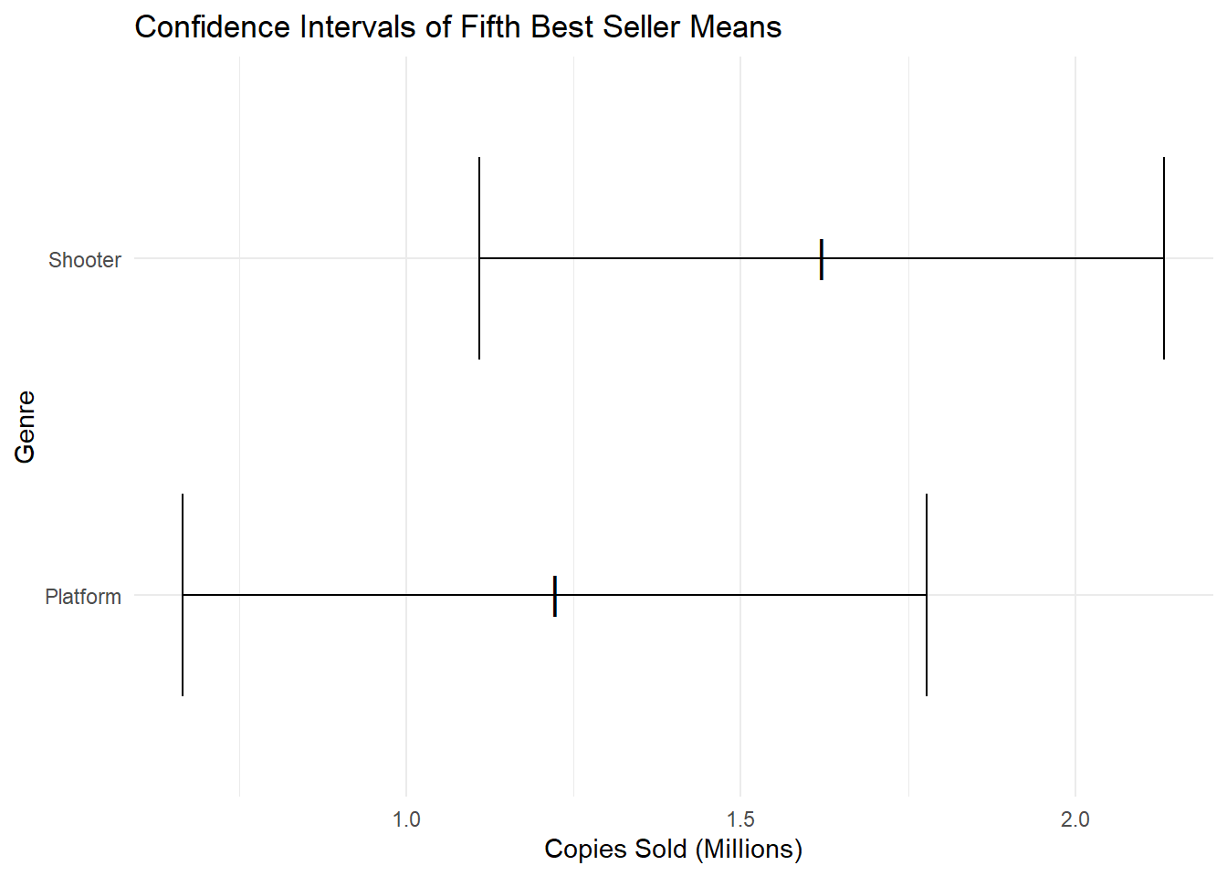
To get an idea of where the fifth-best-sales-mean metric truly falls, we can create confidence intervals around the means calculated from our sample. For both platformers and shooters, we will create a 90% confidence interval, meaning that, if we developed this confidence interval for 100 different samples of our population–assuming our sample is representative of the population–we would expect the true population metric to fall within it 90 times. This does not guarantee our population metric will fall in the interval, but it is generally a reasonable assumption to make. We will assume that our metric follows a normal distribution to determine how many standard errors (calculated from the bootstrapped samples) away from the mean we should use.

Code

P <- 0.9
z_score <- qnorm(p=(1 - P)/2, lower.tail=FALSE)
platform_interval <- game_sales |>
  filter(genre == "Platform") |>
  summarize(lower = fifth_best_platforms_mean - z_score*platform_se,
            upper = fifth_best_platforms_mean + z_score*platform_se)

shooter_interval <- game_sales |>
  filter(genre == "Shooter") |>
  summarize(lower = fifth_best_shooters_mean - z_score*shooter_se,
            upper = fifth_best_shooters_mean + z_score*shooter_se)

intervals <- tibble(genre = c("Platform", "Shooter"),
                    lower = c(platform_interval$lower, shooter_interval$lower),
                    upper = c(platform_interval$upper, shooter_interval$upper),
                    fifth_best_mean = c(fifth_best_platforms_mean,
                                        fifth_best_shooters_mean))

intervals |>
  ggplot() +
  geom_errorbarh(mapping = aes(xmin = lower, xmax = upper, y = genre), height = .6) +
  geom_point(mapping = aes(x = fifth_best_mean, y = genre), shape = '|', size = 6) +
  labs(title = "Confidence Intervals of Fifth Best Seller Means",
       x = "Copies Sold (Millions)", y = "Genre") +
  theme_minimal()

It turns out that the confidence intervals for platformers and shooters have a large amount of overlap. Thus, we cannot make any assumptions about one having a lower fifth best-selling mean statistic than the other. The platformer confidence interval does extend lower than the shooter one, so it may be a better choice for getting our game into the top 5 best-sellers, but we cannot be confident in this assumption.

Conclusions

Although fighting games were the genre preferred by the team, we determined that both platformer and shooter games are probably more likely to reach the necessary sales target of 1.5 million copies sold by using hypotheiss testing. However, there was not a significant difference between platformer and shooter games when it comes to reaching the sales target, and the potential ranges of fifth-best-selling game benchmarks for these two genres overlapped greatly. Platformers may have a lower number of copies necessary to sell in order to reach the top 5 best-sellers of the year, but since we cannot be confident in this, the choice between platformers and shooters can be left up to the development team.

Next Steps

The natural next step for this project would be to gather similar data for games each year up to the present, so the analysis can better reflect current trends in video game sales. Other kinds of data could also potentially be gathered to see if there is a ‘tie-breaker’ that could be used for two genres with similar rates of meeting the sales target and similar fifth-best-seller averages, as seen with Platform and Shooter games above. Information on the development side of video games, such as how long Platform and Shooter games typically take to produce and how much they cost to make, could help determine which is a better choice than the other. Finally, another piece of analysis that could be completed is determining which video game platform would be best for the game to release on by using similar hypothesis testing techniques to those that were used to determine the genre.